Software development

R packages

sBF: Smooth Backfitting
parsec: Partial Orders in Socio-Economics
ineqJD: Inequality Joint Decomposition
POSetR: Partially Ordered Sets in R
HOasso: Higher Order Assortativity for Complex Networks
COGARCH: Simulation and parameters estimation for COGARCH(1,1) processes with different methods

# install.packages("COGARCH", repos="http://R-Forge.R-project.org")

R Programming Examples

Gini Extended index

In this example we evaluate the extended Gini proposed by Yitzhaki in 1983. It is a function of a parameter \(v > 1\) of aversion to inequality and when \(k = 2\) it correspond to the classical Gini index. Its definition is \[ GE(v) = 1 - v(v - 1)\int_0^1 (1 - p)^{v - 2}L(p) dp \] where \(L(p)\) is the Lorenz curve \[ L(p) = \frac{\int_0^p x(p) dp}{\int_0^1 x(p) dp} \] and \(x(p)=\inf\{F(p)\leq p\}\) is the quantile function.

Therefore, in this example is necessary to find the quantile function of a non-negative variable, that can be observed or derived from a distribution model. We choose a Log Normal model with the default values assigned to it by R.

quantile <- qlnorm

but this object can be modified with an another of class function.

Observe that the Lorenz curve is the ratio between the partial integration of the quantile function until p and the whole integration from \(0\) to \(1\). So, before defining the Lorenz curve we evaluate the numerator

q <- Vectorize(\(p) integrate(quantile, lower = 0, upper = p)$value)

using the new introduced \(\lambda\)-function and vectoring the integral by \(p\) so that it can be evaluated for a vector of different upper limits of the integral. Then we define a global variable Q that corresponds to the domination of the Lorenz-curve in order to evaluate it once for all

Q <- q(1)

finally we define the function corresponding to the Lorenz curve

L <- \(p) q(p) / Q

plot(L, xlab = "p", ylab = "L(p)",
  panel.first = lines(c(0, 1), c(0, 1), lty = 2)
)

Finally, we define Gini Extended as an object of class function depending on v

GE <- Vectorize(
  \(v) 1 - v * (v - 1) *
    integrate(\(p) (1 - p)^(v - 2) * L(p),
  lower = 0, upper = 1)$value
)

evaluate it for v equal to \(2\)

G <- GE(2); G

[1] 0.5205004

to get the Gini index, and plot the Gini Extended index as function of v

vmax <- 10
plot(GE, from = 1.001, to = vmax,
     xlim = c(0, vmax),
     ylim = 0:1,
     xlab = "v",
     ylab = "GE(v)"
)
lines(c(0, 2), c(G, G), lty = 2)
lines(c(2, 2), c(0, G), lty = 2)
text(
  c(1, 2),
  c(G + 0.05, 0),
  labels = c(paste("G =", round(G, 2)), "v = 2")
)

Zenga inequality curve decomposition

ineqJD package required

library(ineqJD)

Data simulation

set.seed(23)
n <- 10^4
# vector denoting group membership
G <- sample(1:3, n, replace = TRUE)
# vector of the first source
X1 <- rexp(n)
# vector of the second source
X2 <- rlnorm(n)
data <- data.frame(G, X1, X2)

Decomposition

x <- dataProcessing( # data preparation
  units = data[, c('X1', 'X2')],
  groups = data[, 'G'],
)
decomposition <- zenga(x)
ic <- inequalityCurves(decomposition)
contrib1 <- inequalityCurves(decomposition, l = 1)
contrib12 <- inequalityCurves(decomposition, l = 1:2)

Graphical representation

plot(ic, pch = NULL, lwd = 2)
plot(contrib1, add = TRUE, pch = NULL, lwd = 2, col = 2)
plot(contrib12, add = TRUE, pch = NULL, lwd = 2, col = 3)
text(0.1, 0.1 + 0:2/3, labels = c("G1", "G2", "G3"))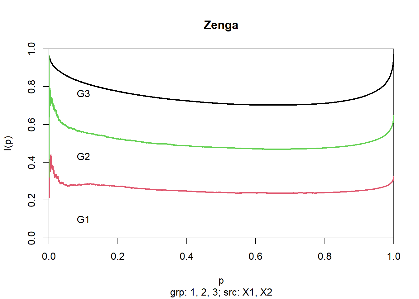

Higher Order Assortativity

Here a simplified description of Higher Order Assortativity assortativity is is shown. In case of undirected and unweighted graphs, assortativity of order \(h=1\) is the correlation between the degrees of adjacent nodes.

igraph package required

library(igraph)

Network creation from adjacency matrix

n <- 5
V <- LETTERS[1:n]
A <- matrix(c(
    0, 1, 1, 0, 0,
    1, 0, 1, 0, 0,
    1, 1, 0, 1, 0,
    0, 0, 1, 0, 1,
    0, 0, 0, 1, 0
  ), nrow = n,
  dimnames = list(from = V, to = V)
)
N <- graph_from_adjacency_matrix(A, mode = "undirected")
plot(N, vertex.color = "white")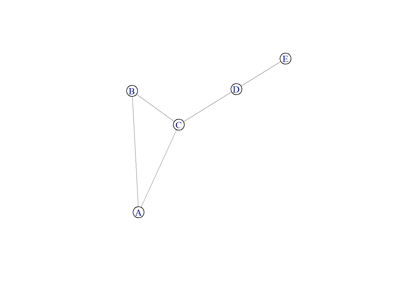

Degree as \(\mathbf{d} = \mathbf{A1}\) centrality measure.

d <- degree(N); d

A B C D E 
2 2 3 2 1

Function to evaluate degree-covariance between joint vertices \[ \text{Cov}(\mathbf{d}, \mathbf{A}) = \mathbf{d}^\top\left(\mathbf{E}-\mathbf{q}\mathbf{q}^\top\right)\mathbf{d} \] where \(\mathbf{E} = \frac{\mathbf{A}}{\|\mathbf{A}\|_1}\) is the relative adjacency matrix and \(\mathbf{q} = \mathbf{E1}\) is the relative degree vector

Cov <- function(d, A) {
  E <- A / sum(A)
  q <- rowSums(E)
  d %*% (E - outer(q, q)) %*% d
}
Cov(d, A)

      [,1]
[1,] -0.04

Assortativity index \[ \rho = \frac{\text{Cov}(\mathbf{d}, \mathbf{A})}{\text{Cov}(\mathbf{d}, \textbf{D}_\mathbf{d})} \] where \(\textbf{D}_\mathbf{d}\) is the diagonal matrix with \(\mathbf{d}\) on the main diagonal

Cov(d, A) / Cov(d, diag(d))

           [,1]
[1,] -0.1111111

Higher order relative adjacency matrix \[ \textbf{E}_h = \textbf{D}_\mathbf{q} \textbf{P}^h \] where \(\textbf{D}_\mathbf{q}\) is the diagonal relative degree matrix and \(\textbf{P}\) is the row-stochastic matrix of the adjacency matrix. If there are not isolated nodes

E <- A / sum(A)
q <- rowSums(E)
D <- diag(q)
P <- solve(D) %*% E
round(P, 3)

      to
           A     B   C     D   E
  [1,] 0.000 0.500 0.5 0.000 0.0
  [2,] 0.500 0.000 0.5 0.000 0.0
  [3,] 0.333 0.333 0.0 0.333 0.0
  [4,] 0.000 0.000 0.5 0.000 0.5
  [5,] 0.000 0.000 0.0 1.000 0.0

rowSums(P)

[1] 1 1 1 1 1

Matrix-power recursive function

matrixPower <- function(M, h) {
  if (h == 1)
    return(M)
  return(M %*% matrixPower(M, h - 1))
}

Assortativity of order \(h = 3\)

P3 <- matrixPower(P, 3)
round(P3, 2)

      to
          A    B    C    D    E
  [1,] 0.17 0.29 0.38 0.08 0.08
  [2,] 0.29 0.17 0.38 0.08 0.08
  [3,] 0.25 0.25 0.17 0.33 0.00
  [4,] 0.08 0.08 0.50 0.00 0.33
  [5,] 0.17 0.17 0.00 0.67 0.00

rowSums(P3)

[1] 1 1 1 1 1

E3 <- D %*% P3
round(E3, 2)

      to
          A    B    C    D    E
  [1,] 0.03 0.06 0.08 0.02 0.02
  [2,] 0.06 0.03 0.08 0.02 0.02
  [3,] 0.07 0.07 0.05 0.10 0.00
  [4,] 0.02 0.02 0.10 0.00 0.07
  [5,] 0.02 0.02 0.00 0.07 0.00

Cov(d, E3) / Cov(d, diag(n))

      [,1]
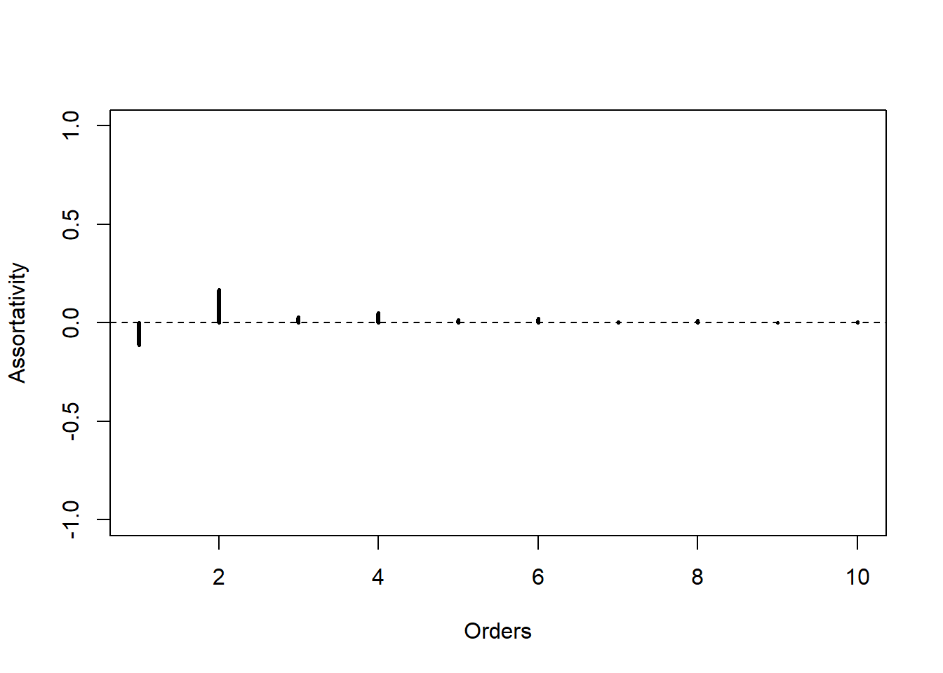
[1,] 0.025

asrt <- Vectorize(
  function(h)
    Cov(d, D %*% matrixPower(P, h)) / Cov(d, diag(n))
)
plot(asrt(1:10), type = "h", xlab = "Orders",
  ylab = "Assortativity", lwd = 3, ylim = c(-1, 1),
  panel.first = abline(h = 0, lty = 2)
)

Using `HOasso` package

The package allows the evaluation of Higher Order Assortativity for digraphs and weighted graphs too, but in this case we refer to the previous example, undirected and unweighted, in order to show how to get the same results using only one function.

library(HOasso)

a <- HOasso(N, h = 10)
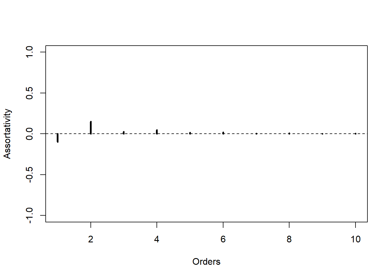
class(a)

[1] "assortativity" "numeric"

The result is an object of class assortativity with its own methods but it hinerits the properties of numeric vectors.

print(a)

     
order assortativity
   1   -0.111111111
   2    0.166666667
   3    0.027777778
   4    0.050925926
   5    0.016203704
   6    0.021990741
   7    0.005594136
   8    0.010898920
   9    0.001012731
   10   0.005875450

plot(a, lwd = 3, panel.first = abline(h = 0, lty = 2))